


Washington vs. Oregon - 2024 Edition

As a graduate of the University of Washington (and life member of the UW Alumni Association), I have an undeniable personal/emotional investment in the annual grudge match that is my undergraduate alma mater playing our hated enemy, the University of Oregon.

Meme that came out last year after we beat them twice!
This year’s matchup is the 117th between UW & U of O, and it should be noted, all-time, Washington leads in this rivalry, 63–48–5 (.565).
[For my readers solely here for med school pathway oriented content, I apologise & feel free to ignore this. For anyone interested in sports, I hope you enjoy the following.]
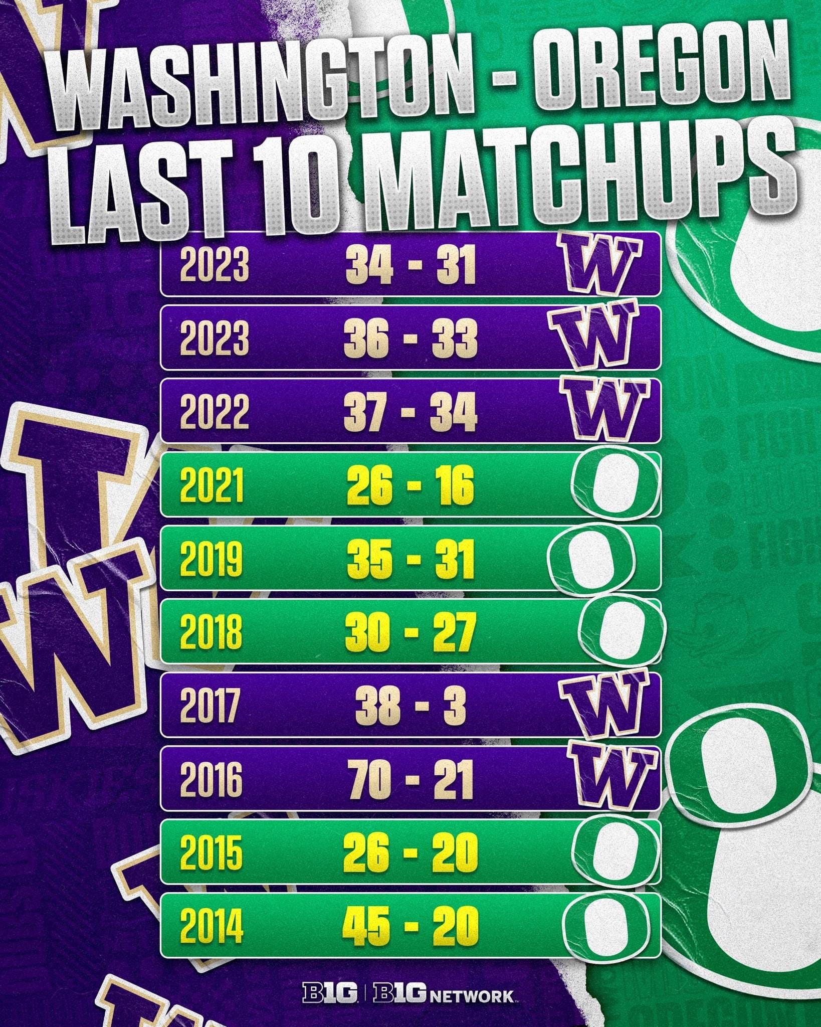
To estimate the results for the upcoming Huskies vs. Ducks game (we really need a cool name for it), I looked at the last 10 matchups, current team statistics for this season, and home-field advantage dynamics.
With credit given to Bill Scherer & my time in government, let me lead off with the results I expect, considering all factors:
Oregon 31, Washington 19
(Amended after fixing an error in my work earlier, this brings down the estimated results for both teams, and brings the estimated result to under the betting line)
Summary of why I expect this:
• Oregon’s offensive and defensive advantages, combined with Washington’s defensive vulnerabilities, should result in a comfortable win for the Ducks.
• This predicted margin aligns with a bit less than the current betting spread (-19 for Oregon according to what I saw on ESPN) as well as reflects the significant impact of home-field advantage (which I estimate at 6-9 points, a figure that ChatGPT agrees with, which is a lesser figure than I originally computed, due to an error I made in transcribing team scores for the 2016 game).
Key Observations from the Data
1. Historical Matchups:
• Washington and Oregon have alternated wins recently, but Oregon has generally had more dominant victories during this period, especially at Autzen Stadium. A notable exception was Washington's emphatic 70-21 victory at Autzen in 2016, highlighting their potential to excel under the right circumstances.
• Washington’s wins, particularly in 2022 and 2023, have been narrow and often decided by fewer than a touchdown.
2. Current Season Performance:
• Oregon is 11-0 overall and 8-0 in conference play, demonstrating dominance both offensively and defensively (263 points scored vs. 111 allowed in conference play).
• Washington is 6-5 overall and 4-4 in conference, with a weaker defence (189 points allowed in conference play) and only a marginal scoring edge in total games (249 scored vs. 225 allowed).
3. Home-Field Advantage:
• Autzen Stadium has a reputation for being one of the loudest and most intimidating environments in college football.
• Historically over the last bunch of years, Oregon has performed significantly better at home in Autzen Stadium against Washington compared to games in Husky Stadium in Seattle.
4. Betting Lines and Predictions:
• Oregon is favoured by 19 points, with an 88.8% win probability according to ESPN analytics. This suggests a high level of confidence in Oregon’s ability to dominate.
5. Player Matchups:
• Oregon’s offensive leaders (Gabriel, James, Johnson) are statistically stronger than Washington’s counterparts.
• Washington has a strong rushing game with Coleman, but Oregon’s balanced offence (passing and rushing) will likely exploit Washington’s defence.
Home-Field Advantage Estimation
• Historically, Oregon has demonstrated strong performance at Autzen Stadium, with notable victories such as 45-20 in 2014. However, Washington's 70-21 win at Autzen in 2016 tempers the notion of an impenetrable home-field advantage.
• In comparison, games in odd years at Husky Stadium or neutral sites are closer contests, often decided by single digits.
• Based on this trend, home-field advantage for Oregon appears to be worth approximately 6-9 points, reflecting historical trends and Washington's potential to neutralise the advantage, as seen in 2016.
I wish it was otherwise, and we won’t actually know what happens until Saturday night (if models were 100 per cent effective, we’d never actually need to play the games), but it looks like it’s going to be a rough night for my beloved Huskies.
For anyone interested in a deeper dive into the statistics regarding performance by location in the Huskies vs. Zeroes games, let me share the table of results from Wikipedia.
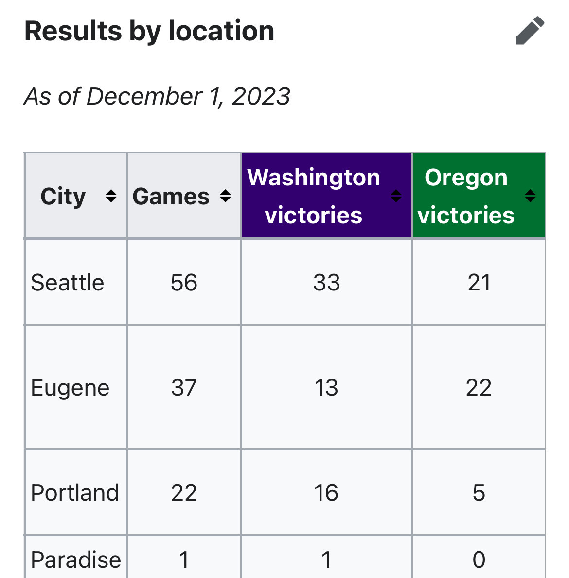
From this, we know the following:
Conducting a chi-square test on the all-time performance data by location.
The important results are:
• Chi-square statistic: 9.90
• P-value: 0.019
• Degrees of freedom: 3
The P-value suggests that there is a statistically significant difference in win distributions by location at a 5% significance level.
Here’s a more detailed interpretation and analysis of the chi-square test and the data:
1. Hypotheses
• Null Hypothesis (H_0): The distribution of wins (Washington vs. Oregon) is independent of the game location.
• Alternative Hypothesis (H_a): The distribution of wins (Washington vs. Oregon) depends on the game location.
2. Test Results
• Chi-square statistic: 9.90
• P-value: 0.019
• Degrees of freedom: 3
• Significance level: 0.05
Since the P-value (0.019) is less than the significance level (0.05), we reject the null hypothesis. This indicates that the win distribution between Washington and Oregon is not independent of location. In simpler terms, location significantly influences the win outcomes.
3. Expected Frequencies
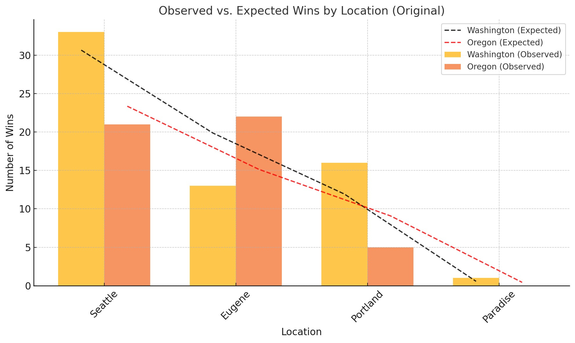
The expected frequencies demonstrates how wins would have been distributed if location had no effect (based solely on the total number of games and wins).
Here’s a breakdown by location:
• Seattle: Washington wins more often than expected (33 vs. 30.65), while Oregon wins less than expected (21 vs. 23.35).
• Eugene: Oregon wins significantly more often than expected (22 vs. 15.14), while Washington wins less than expected (13 vs. 19.16).
• Portland: Washington exceeds expectations significantly in neutral-site games (UW: 16 vs. 11.92, U of O: 5 vs 9.08).
• Paradise: Too small a sample size to draw meaningful conclusions (UW: 1 vs. 0.57, U of O: 0 vs. 0.43)
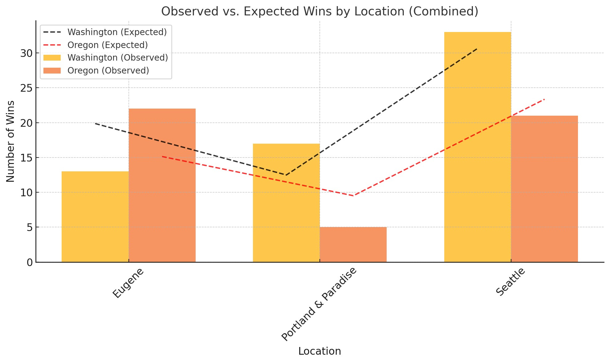
Even when combining Portland and Paradise into a single category as “neutral site”, the statistical results differ slightly:
A. Original Analysis (Separate Portland and Paradise, as I share above):
• Chi-square statistic: 9.90
• P-value: 0.019
• Degrees of freedom: 3
2. Combined Analysis (Portland & Paradise combined):
• Chi-square statistic: 9.68
• P-value: 0.0079
• Degrees of freedom: 2
Observations Between These Two:
• Chi-square statistic: Slightly reduced when combining locations, but still significant.
• P-value: Becomes more significant (lower) in the combined analysis, suggesting stronger evidence that location influences game outcomes.
4. Main Observations Across Scenarios
• Seattle advantage for Washington: Washington overperforms at home, winning more games than expected. This aligns with the historical trend that home-field advantage is real for the Huskies.
• Eugene advantage for Oregon: Oregon dominates at Autzen Stadium, significantly outperforming expectations. This reinforces the notion of Eugene as a difficult place for Washington to win.
• Portland as a neutral site: Washington has historically done better than expected here, suggesting that removing the home-field advantage from either team slightly favours Washington.
• Paradise: With just one game, there is insufficient data to analyse trends ergo why I did the combined analysis as well.
Lastly, the code in Python for those interested (developed with assistance from ChatGPT):
Original work:
import pandas as pd
from scipy.stats import chi2_contingency
# Data from the table
data = {
"City": ["Seattle", "Eugene", "Portland", "Paradise"],
"Games": [56, 37, 22, 1],
"Washington_wins": [33, 13, 16, 1],
"Oregon_wins": [21, 22, 5, 0]
}
# Create a DataFrame
df = pd.DataFrame(data)
# Perform chi-square test
contingency_table = df[["Washington_wins", "Oregon_wins"]].values
chi2, p, dof, expected = chi2_contingency(contingency_table)
# Store results
results = {
"Chi-square statistic": chi2,
"P-value": p,
"Degrees of freedom": dof,
"Expected frequencies": expected
}
import ace_tools as tools; tools.display_dataframe_to_user(name="All-Time Performance Analysis by Location", dataframe=pd.DataFrame(results["Expected frequencies"], columns=["Washington (expected)", "Oregon (expected)"], index=df["City"]))
results
Work with Combined Neutral Location
# Combine Portland and Paradise into a single category
df_combined = df.copy()
df_combined.loc[df_combined["City"].isin(["Portland", "Paradise"]), "City"] = "Portland & Paradise"
df_combined = df_combined.groupby("City").sum().reset_index()
# Perform chi-square test for the combined category
contingency_table_combined = df_combined[["Washington_wins", "Oregon_wins"]].values
chi2_combined, p_combined, dof_combined, expected_combined = chi2_contingency(contingency_table_combined)
# Prepare combined results for comparison
comparison_results = {
"Original Chi-square statistic": chi2,
"Original P-value": p,
"Original Degrees of freedom": dof,
"Combined Chi-square statistic": chi2_combined,
"Combined P-value": p_combined,
"Combined Degrees of freedom": dof_combined
}
tools.display_dataframe_to_user(
name="Expected Frequencies with Combined Locations",
dataframe=pd.DataFrame(expected_combined, columns=["Washington (expected)", "Oregon (expected)"], index=df_combined["City"])
)
comparison_results
Work with Data Visualisation
import matplotlib.pyplot as plt
import numpy as np
# Visualising the data
# Bar chart for observed vs. expected wins (original)
fig, ax = plt.subplots(figsize=(10, 6))
width = 0.35 # Bar width
locations = df["City"]
x = np.arange(len(locations))
# Observed values
ax.bar(x - width/2, df["Washington_wins"], width, label="Washington (Observed)", alpha=0.7)
ax.bar(x + width/2, df["Oregon_wins"], width, label="Oregon (Observed)", alpha=0.7)
# Expected values
expected_original_df = pd.DataFrame(expected, columns=["Washington", "Oregon"], index=locations)
ax.plot(x - width/2, expected_original_df["Washington"], 'k--', label="Washington (Expected)", alpha=0.8)
ax.plot(x + width/2, expected_original_df["Oregon"], 'r--', label="Oregon (Expected)", alpha=0.8)
# Formatting
ax.set_xlabel("Location", fontsize=12)
ax.set_ylabel("Number of Wins", fontsize=12)
ax.set_title("Observed vs. Expected Wins by Location (Original)", fontsize=14)
ax.set_xticks(x)
ax.set_xticklabels(locations, rotation=45)
ax.legend()
plt.tight_layout()
plt.show()
# Pie chart showing proportion of Washington vs. Oregon wins (overall)
total_wins = df[["Washington_wins", "Oregon_wins"]].sum()
labels = ["Washington", "Oregon"]
colors = ["purple", "green"]
plt.figure(figsize=(8, 6))
plt.pie(total_wins, labels=labels, autopct='%1.1f%%', startangle=90, colors=colors)
plt.title("Overall Win Proportions: Washington vs. Oregon", fontsize=14)
plt.show()
# Combined analysis bar chart
fig, ax = plt.subplots(figsize=(10, 6))
locations_combined = df_combined["City"]
x_combined = np.arange(len(locations_combined))
# Observed values for combined
ax.bar(x_combined - width/2, df_combined["Washington_wins"], width, label="Washington (Observed)", alpha=0.7)
ax.bar(x_combined + width/2, df_combined["Oregon_wins"], width, label="Oregon (Observed)", alpha=0.7)
# Expected values for combined
expected_combined_df = pd.DataFrame(expected_combined, columns=["Washington", "Oregon"], index=locations_combined)
ax.plot(x_combined - width/2, expected_combined_df["Washington"], 'k--', label="Washington (Expected)", alpha=0.8)
ax.plot(x_combined + width/2, expected_combined_df["Oregon"], 'r--', label="Oregon (Expected)", alpha=0.8)
# Formatting
ax.set_xlabel("Location", fontsize=12)
ax.set_ylabel("Number of Wins", fontsize=12)
ax.set_title("Observed vs. Expected Wins by Location (Combined)", fontsize=14)
ax.set_xticks(x_combined)
ax.set_xticklabels(locations_combined, rotation=45)
ax.legend()
plt.tight_layout()
plt.show()
Home Field Advantage Revision & Revised Final Score Computation
# Data for Washington and Oregon's performance this season (conference data as a base)
oregon_points_scored = 263 # Conference points scored
oregon_points_allowed = 111 # Conference points allowed
oregon_games = 8 # Conference games
washington_points_scored = 165
washington_points_allowed = 189
washington_games = 8
# Calculate average points per game
oregon_avg_scored = oregon_points_scored / oregon_games
oregon_avg_allowed = oregon_points_allowed / oregon_games
washington_avg_scored = washington_points_scored / washington_games
washington_avg_allowed = washington_points_allowed / washington_games
# Include the spread and over/under as external inputs
spread = 19 # Oregon favored by 19
over_under = 50.5
# Historical Eugene scoring trends from the last 10 matchups in Eugene
# Wins at Autzen: Oregon typically scored more points at home, but we need to reflect the 2016 anomaly
historical_eugene_oregon_avg = (45 + 21 + 26 + 35) / 4 # Oregon points (excluding neutral-site years)
historical_eugene_washington_avg = (20 + 70 + 16 + 13) / 4 # Washington points
# Weighted adjustments based on season averages and historical trends
oregon_weighted_score = (oregon_avg_scored * 0.6) + (historical_eugene_oregon_avg * 0.4)
washington_weighted_score = (washington_avg_scored * 0.6) + (historical_eugene_washington_avg * 0.4)
# Adjust for Oregon's home-field advantage
home_field_advantage = 6.5 # Revised value
oregon_final_score = oregon_weighted_score + home_field_advantage
washington_final_score = washington_weighted_score
# Adjust for the over/under total to normalise the final output
total_points = oregon_final_score + washington_final_score
scaling_factor = over_under / total_points
# Apply scaling factor to normalize to the betting over/under
oregon_final_score_scaled = oregon_final_score * scaling_factor
washington_final_score_scaled = washington_final_score * scaling_factor
oregon_final_score_scaled, washington_final_score_scaled
And that’s a full lid, folks!
Note: This post was updated to correct an error in the historical scoring data for the 2016 matchup, which originally attributed a 70-21 score to Oregon instead of Washington. The revised prediction and analysis reflect this correction, thanks be to my friend Brad Jacobsmeyer who pointed it out. It was also revised to fix a couple of minor spelling and grammar errors - downside for me using the Substack app to type out a post, but still, not bad to use on the whole.